Analyzing learning rates (pt. 2): Two approaches

TL/DR

• Modelling and comparing learning curves is difficult because (i) most learning curves are non-linear and (ii) most methods of modelling non-linear curves use multiple parameters to describe learning. How do you holistically compare learning curves described by multiple parameters (e.g., think about a quadratic regression)? The power-law function can be useful to address this problem, while also accurately depicting most learning trajectories.
• Explicit modelling of the learning curves can be avoided by instead comparing groups based on average performance or performance after a learning period (like a final exam). These methods can work nicely, but only when initial performance is the same across groups.

Overview

This blog entry is part two of two on how to analyze learning. Reading part one will help in understanding part two, but it is not necessary. Recall that part one outlined issues that can arise when comparing learning curves. The main challenge lies in modeling both when learning occurs (i.e., earlier versus later) and how much total learning has occurred (i.e., the difference in knowledge or performance at the end compared to the beginning). This post discusses various approaches to dealing with those challenges along with the pros and cons of these approaches. The first class of approaches focus on modelling the learning curves – estimating the changes in performance. The second class of approaches do not look at changes, but instead examine overall performance or performance at one point-in-time after a learning period.

Approach #1: Modelling and Comparing Learning Curves

Perhaps the most obvious approach to examining learning is to explicitly model and then compare the different learning curves. The shape of a learning curve represents when the learning occurs (e.g., concavity implies early learning; convexity implies later learning; and linearity implies constant learning).¹ The average slope of each curve represents how much total learning has occurred. This modelling approach can be difficult because aggregate learning curves are almost always non-linear (Argote and Epple 1990; Donner and Hardy 2015; Gallistel, Fairhurst, and Balsam 2004; Haider and Frensch 2002; Wright 1936), which presents two main challenges: 1) estimating the curve appropriately and 2) using an estimation method that allows comparisons between curves.

Polynomial Regression

Polynomial regression is one method of modelling non-linear curves. This method can work, but there are two major issues. First, most learning curves are not polynomial (more on this later). Second, how do you compare learning? Consider using a quadratic regression to model two learning curves: A and B. If curve A has a more positive coefficient than curve B on both the linear and quadratic term, then you can say with some certainty that curve A represents better learning. But what if one coefficient is more positive while the other is more negative (as is often the case)? The main issue is that with the quadratic regression, two coefficients jointly capture learning such that we do not have a holistic comparison. This issue grows exponentially (pun intended) with the polynomial degree. If we only need to model the learning curve, then the polynomial regression might work. But when comparing learning curves, what we really want is a model that gives one statistical term to completely describe learning in each curve, allowing a clean comparison.²

Power-Law
In this vein, prior research often uses the power-law function (Argote and Epple 1990; Haider and Frensch 2002; Levitt, List, and Syverson 2013; Wright 1936):

$$y = a \times x^k$$

The first term ($a$) gives the y-intercept, i.e., performance when $x$ is zero. The second term ($k$) gives the growth rate. This growth rate determines the percentage increase in performance from trial $x$ to trial $x+1$.³ Thus, we have one term for the starting point ($a$) and one term for the change across trials ($k$). Voila! The growth rate $k$ provides a single term that represents learning! Appendix A describes how to estimate power-law regressions in Stata.

There are two other benefits of using the power-law function. First, it accurately depicts most aggregate learning curves (Argote and Epple 1990; Haider and Frensch 2002; Wright 1936).⁴ Second, it can flexibly capture growth – by giving $k$ a positive value – and decay – by giving k a negative value.⁵ The maximum-likelihood parameter estimation in Stata will naturally determine whether k should be positive or negative. See Samet, Schuhmacher, Towry, and Zureich (2022) for an example use of the power-law function for comparing non-linear decay across groups.

Percentage versus Absolute Changes

There is one key caveat to the power-law approach: the growth rate indicates the percentage change from one trial to the next rather than the absolute change. A higher percentage growth rate typically coincides with a higher absolute change, but not always because learning curves may differ in their starting point. If one curve starts at a low performance level (e.g., 10), then a large percentage increase (e.g., 50) from that low level may correspond to a small absolute change (5 = 10 $\times$ 50%). In contrast, if one curve starts at a high performance level (e.g., 100), then a small percentage increase (e.g., 10%) from that high level may correspond to a large absolute change (10 = 100 $\times$ 10%).⁶ Eventually, the curve with the larger growth will catch up – no matter the starting point – but this may not show in the data. Thus, the starting point, i.e., the y-intercept (a), might matter when considering absolute changes but not when considering percentage changes. Growth rate as a percentage change is a commonly used metric, but the appropriateness of relying on percentage or absolute changes depends on the research question and setting. When absolute changes do matter, then we again run into the issue of having to compare learning curves based on multiple parameters (a and k in this case). But when percentage changes matter, the issue is avoided. Similar ideas also apply to other growth and decay models (e.g., exponential decay models).

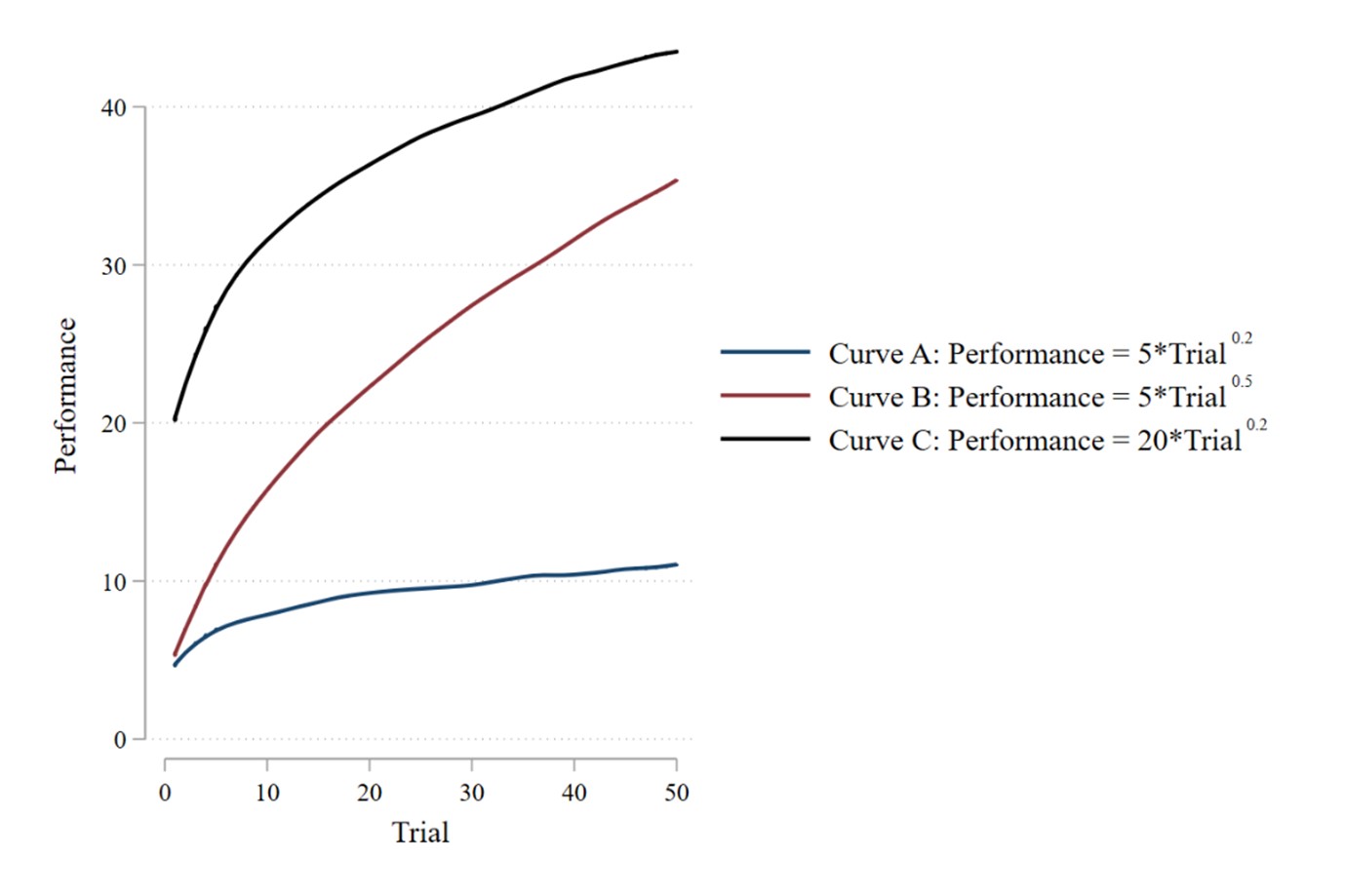
To make these ideas more concrete, consider the three example learning curves below with their respective power-law estimations. First note that B has a higher growth rate than both A (0.5 vs. 0.2) and C (0.5 vs. 0.2). As expected, B increases more from start to finish than A, both in terms of absolute change (30.36 increase vs. 5.98 increase) and percentage change (604% vs. 120%). However, interestingly, B increases less than C in terms of absolute change (30.36 increase vs. 38.72 increase) but more than C in terms of percentage change (604% vs. 119%). This pattern occurs because B has a higher growth rate but a lower starting point than C. Curves with higher growth rate will always eventually surpass those with lower growth rates, but this may not be observed within the time span of the study.

There are certainly other approaches to modelling curves, like using spline regressions (Marsh and Cormier 2001). However, these approaches typically use multiple parameters to model the curves, giving the issue of how to make a holistic comparison. Overcoming this issue (at least partially) is a benefit of the power-law approach.

Approach #2A: Examine overall performance instead of “learning”

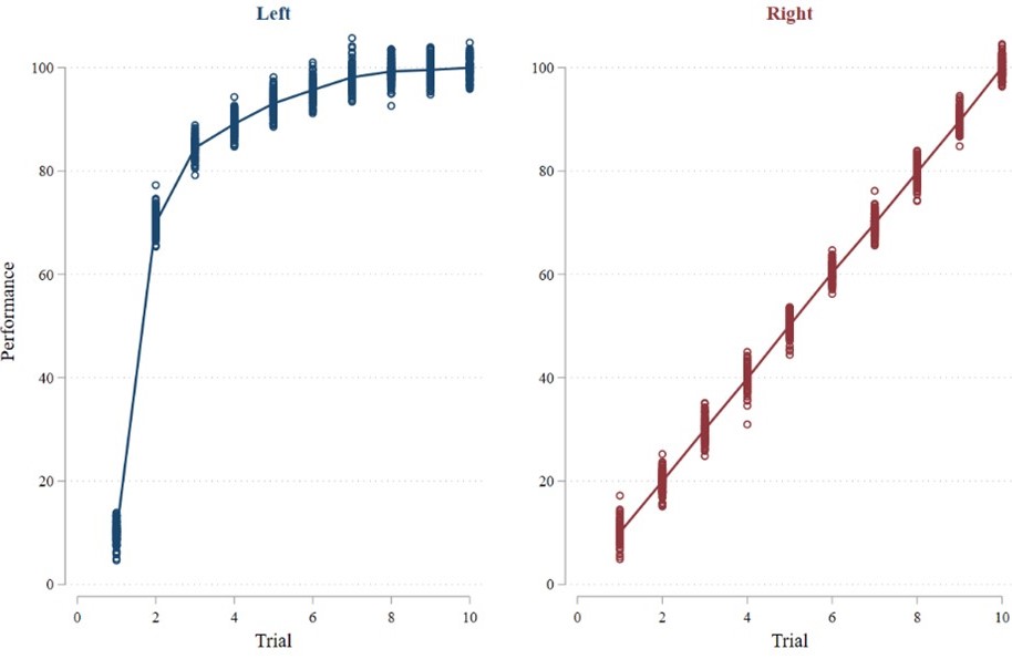
Rather than modelling changes in performance across trials, researchers can instead examine total performance as a proxy for learning. The idea is that if individuals in situation A learn better than individuals in situation B, then those in situation A will have higher performance on average. Consider the two graphs from the previous post (and reproduced below). Clearly, average performance is higher in the left graph than in the right graph.⁷ Thus, in contrast to the two approaches outlined in the previous post, examining total performance accurately reflects the better learning given in the left graph. Great – the previously outlined issues seem to be fixed! But, can we always expect this approach to work? If not, when will it work and why?⁸

Average Performance = 83.92	Average Performance = 54.96

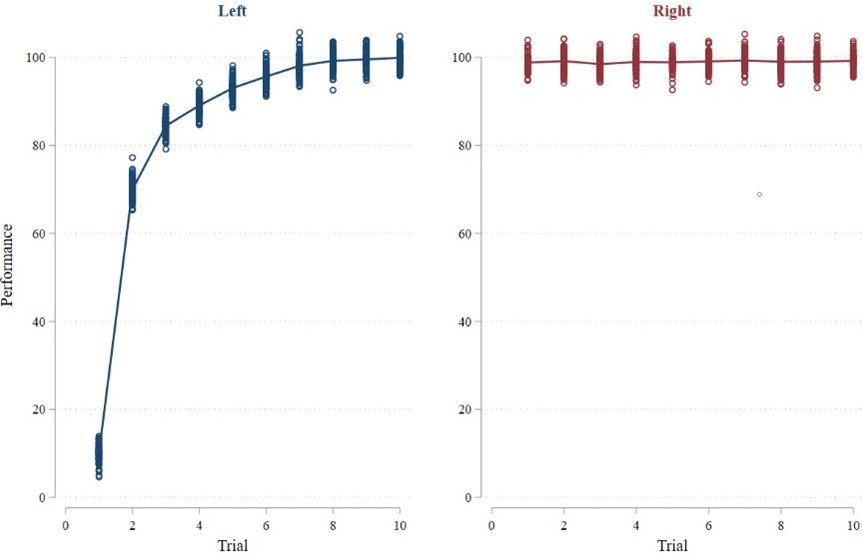
The key assumption with this approach is that the two groups being compared have the same initial performance. In an experiment, this means that the manipulations cannot affect initial performance. If this assumption is not met, then one group can have higher average performance without improving more across trials simply because that group had better performance initially. For example, if our learning curves instead look like the two curves below, then the average performance approach will favor the graph on the right even though we can still clearly see that there is better learning in the graph on the left.

Average Performance = 83.92	Average Performance = 99.02

How do we know whether the experimental manipulations affect initial performance and, more generally, when can we theoretically expect this to be case? The answer to the first question is seemingly straightforward – simply compare performance on the first trial. However, using only the first trial might be a low powered test, and there could be arguments to use the first two, three, or five trials. Stated differently, what block of trials constitutes “initial performance?” Another problem is that this comparison of initial performance relies on null evidence.

A better solution is to argue theoretically that initially performance cannot differ across groups. Such an argument can be made using carefully constructed experimental tasks. In particular, the manipulations cannot affect initial performance when participant are given no prior information about which actions are best initially, and their prior experiences outside the lab in no way help them know which actions are best initially. In these cases, participants can only guess at first. Assuming the manipulations do not affect how accurately people guess, then initial performance should be the same on average. A nice example is the classic multi-armed bandit task. Consider the 2-armed version of this task in which participants repeatedly choose between two options: A and B. Participants can only learn the value of each option by choosing the option and observing the noisy reward it provides. On the first trial, they have no idea which option is better and can only guess. The manipulations can therefore have no possible effect on initial performance. Only over time can participants perform better than randomly guessing by learning the reward distributions for the two buttons after repeatedly sampling from them.

Approach #2B: Examine learning at the end (the “Final Exam” approach)

Another common approach is to examine performance after a pre-specified learning period (e.g., Merlo and Schotter 1999, 2003; Thornock 2016). For example, Choi, Hecht, Tafkov, and Towry (2020) examines participants’ performance on trial 36 of their experimental task, which captures how much individuals learned in total from trials 1 through 35. I call this the “Final Exam” approach because it tests (in an incentive compatible way) how much knowledge or skill individuals have accumulated after a period of time.

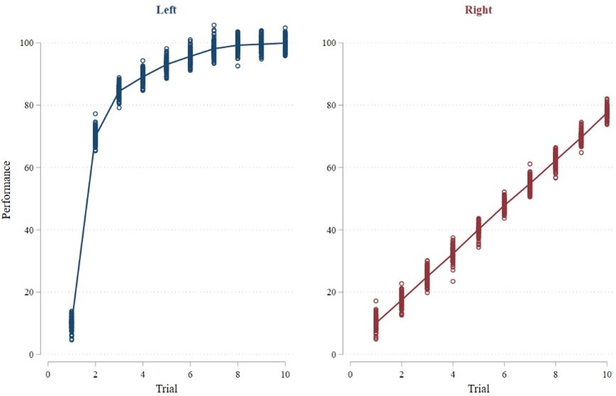
While the Final Exam approach is certainly valid and useful, it should be noted that it generally ignores when the learning occurs and instead asks how much individuals have learned after a set amount of experience. That is, by examining learning only after the learning period, it is clear how much individuals have learned in sum but not how quickly they got to that point during the learning period. This is not a criticism of the Final Exam approach. Rather, it is an understanding of what this approach does and does not capture. Total learning after a prespecified learning period is certainly a useful metric when studying learning! And in many cases, those who learned the most after a set period of trials probably also learned more quickly. However, this need not always be the case. For example, the final exam approach would not identify learning differences in the two learning curves from the original post (see Figure B above) because performance in the final trial is equal in both curves. Yet this is an artificial example. A more plausible variation on that example is where the second curve closes the gap with the first curve, but not all the way (see Figure D below). In this new example, the final exam approach would work fairly well whereas the two approaches from the first post (i.e., linear regression and 2nd half minus 1st half performance) would still fail.

Average Performance = 99.95	Average Performance = 77.55

Three other factors are important to consider with this approach.

First, this approach also assumes that initial performance is the same across groups. Think about two identical sections of a business course. One is taken by first-year students and the other by third-year students. Comparing the courses based on the final exam is unfair because one group came in with more knowledge than the other. Thus, one group might perform better than another after the learning period because they started better, even if they did not improve as much throughout the task. Smartly, prior studies use abstract tasks in which prior knowledge plays little role and initial performance essentially amounts to guessing.

Second, the incentive structure matters (Merlo and Schotter 1999). Prior studies typically use weak incentives, or even no incentives, in the learning period and then give strong incentives for performance in the final period (i.e., the final exam). This choice to use weak incentives is important because it encourages participants to experiment in the learning period and can affect how they frame the learning task. If incentives are strong in the learning period, then participants may learn reactive strategies (e.g., win stay-lose shift) rather than trying to learn optimal strategies. Similarly, strong incentives can also cause participants to make choices that maximize current performance rather than choices that would give the most information for the final exam. That is, when incentives are strong, participants need to manage the explore-exploit tradeoff, and differences in the way they manage this tradeoff affects the information they will have observed when it comes time for the final exam. Thus, when incentives are strong, there may be differences in learning due to differences in the way participants manage the explore-exploit tradeoff (Ederer and Manso 2013; Manso 2011; March 1991; Merlo and Schotter 1999). Whether these effects are desirable or undesirable depends on the research question, but the point remains that incentives during the learning period are important to consider.⁹

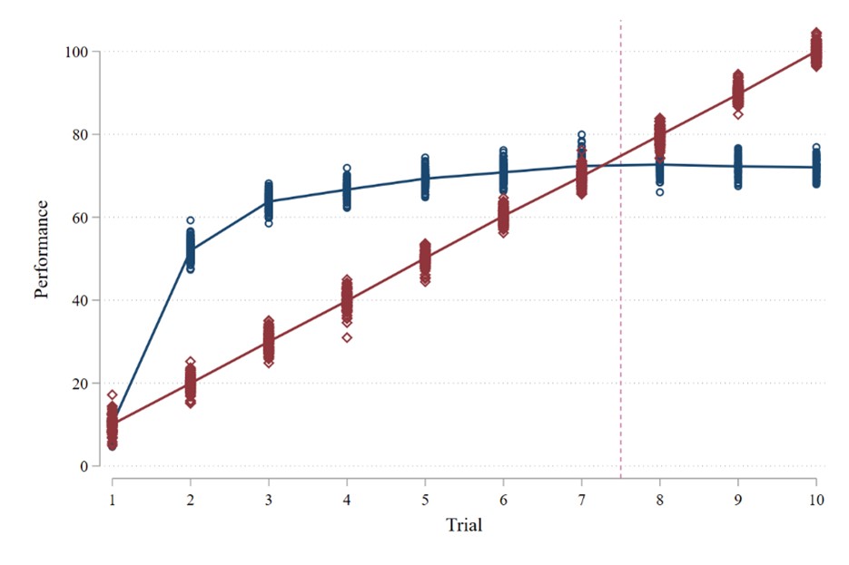
Third, the length of the learning period also matters. For example, consider the two learning curves below. The blue curve depicts quick initial learning that tapers off (i.e., a concave learning curve representing diminishing returns to experience). The red curve depicts steady learning that ultimately exceeds he other group (i.e., a linear learning curve representing constant returns to experience). The length of the learning period determines which of these groups appears to have learned more on the final exam. If the learning period is seven or fewer trials – meaning the final exam occurs somewhere before trial eight – then the group depicted by the blue curve will appear to have learned more. However, if the learning period is eight or more trials, then the group depicted by the red curve will appear to have learned more. This is similar to the discussion of absolute changes with the power-law function, where curves with lower starting points but higher growth rates will eventually catch up to curves with higher starting points but lower growth rates.

Conclusion

In sum, there are two classes of approaches to analyze learning: the first class explicitly models the learning curves whereas the second class does not model the curves. The power-law function is useful for the first class of approaches because it accurately describes most aggregate learning curves and gives one parameter to describe learning (the growth rate). The second class of approaches are simpler, but they rest on the assumption that initial performance does not differ across groups. Differences in initial performance can be compared, but an even nicer solution for experimentalists is to use abstract tasks in which the manipulations can in no way affect initial performance.

Appendices

Appendix A describes how to estimate power-law regressions in Stata.

References

How to reference this online article?